Chapter 3- False Nearest Neighbours and Embedding Dimensions

We employed a technique known as false nearest neighbors (FNN), introduced by Kennel et al.(1992), to ascertain the minimum number of dimensions needed to faithfully reconstruct an attractor. An attractor serves as a representation of how a system evolves over time.

In our analysis, our goal was to ensure that when we represent this evolution in lower dimensions, we do not lose crucial details. False nearest neighbors play a crucial role in this determination. They are points that may seem close together in a lower-dimensional depiction but are actually distant in the original higher-dimensional space.

To illustrate, consider trying to draw a detailed picture of a tree on a small piece of paper. You might find it challenging to capture all the branches and leaves due to space constraints. Similarly, in our analysis, starting with a lower-dimensional representation of the system’s behavior may obscure important details. This situation is akin to trying to fit a detailed tree drawing on a tiny piece of paper – some parts may appear connected, but they are distinct.

Identifying many false nearest neighbors suggests that our lower-dimensional representation lacks essential information. Increasing the dimensions allows us to “unfold” the attractor and separate these falsely identified neighbors. This process ensures that our representation accurately captures the system’s dynamics. Hence, false nearest neighbors serve as a guide to determine if our chosen dimensions adequately represent the complete picture of the system’s behavior over time.

In simpler terms, let’s say we have a time series with an ideal embedding dimension of \(m_0\). When we reduce the dimension by one, some points are strongly affected and become false nearest neighbors (FNN). To identify these FNN points, we compared the distances between points in the \(m\)-dimensional space with those in the \(m+1\)-dimensional space and calculated their ratio.

\[X_{fnn}(r) = \frac{\sum_{n=1}^{N-m-1} \Theta\left(\frac{|x_n^{(m+1)}-x_{k(n)}^{(m+1)}|}{|x_n^{(m)}-x_{k(n)}^{(m)}|}-r\right) \Theta\left(\frac{\sigma}{r}-|x_n^{(m)}-x_{k(n)}^{(m)}|\right)}{\sum_{n=1}^{N-m-1}\Theta\left(\frac{\sigma}{r}-|x_n^{(m)}-x_{k(n)}^{(m)}|\right)}\]

Where :math:` x_{k(n)}^{(m)}` represents the nearest neighbor of \(x_n^{(m)}\) in \(m\) dimensions, and \(\Theta(x)\) denotes the Heaviside step function. \(\sigma\) signifies the standard deviation of the data. The function \(k(n)\) is defined as follows:

\[k(n) = \{ n' \mid |x_n^{(m)} - x_{n'}^{(m)}| \leq |x_n^{(m)} - x_{n''}^{(m)}|, \forall n'' \in I(x) - n \}\]

where \(I(x)\) is the set of all indices of x. k(n) is estimated using nearest() function in the package

nearest()

nearest(s, n, d, tau, m)

Function that would give a nearest neighbour map, the output array(nn) stores indices of nearest neighbours for index values of each observations

Parameters:

• s (ndarray) – 3D matrix ov size ((n-(m-1)*tau,m,d)), time delayed embedded signal

• n (int) – number of samples or observations in the time series

• d (int) – number of measurements or dimensions of the data

• tau (int) – amount of delay

• m (int) – number of embedding dimensions

Returns:

nn (array) – an array denoting index of nearest neighbour for each observation

References

• Takens, F. (1981). Dynamical systems and turbulence. Warwick, 1980, 366–381.

A more appropriate method would be to see the FNN ratio as a function of r (see Kantz and Schreiber(2004), section 3.3.1, page 37, figure 3.3)) if we are interested in parameter exploration.

For this we defined the radius at which FNN hist zero as:

\[r_0(m) = \{ r \mid X_{fnn}(r) < \delta, \forall r \in [r_{\min}, r_{\max}] \}\]

Where \([r_{min},r_{max}]\) is the interval where we are searching, which is for m embedding dimensions, and \(\delta\) is a small enough number. This was implemented using the function fnnhitszero()

fnnhitszero()

fnnhitszero(u, n, d, m, tau, sig, delta, Rmin, Rmax, rdiv)

Function that finds the value of r at which the FNN ratio can be effectively considered as zero

Parameters:

• u (ndarray) – double array of shape (n,d). Think of it as n points in a d dimensional space

• n (int) – number of samples or observations in the time series

• d (int) – number of measurements or dimensions of the data

• tau (int) – amount of delay

• m (int) – number of embedding dimensions

• r (double) – ratio parameter

• sig (double) – standard deviation of the data

• delta (double) – the tolerance value(the maximum difference from zero) for a value of FNN ratio to be effectively considered to be zero

• Rmin (double) – minimum value of r from where we would start the parameter search

• Rmax (double) – maximum value of r for defining the upper limit of parameter search

• rdiv (Int) – number of divisions between Rmin and Rmax for parameter search

Returns:

r (double) – value of r at which the value of FNN ratio effectively hits zero

References

• Kantz, H., & Schreiber, T. (2004). Nonlinear time series analysis (Vol. 7). Cambridge university press. section 3.3.1

When doing this for different values of embedding dimensions, we will get r values which when ploted against corresponding embedding dimension would look like the following figure:

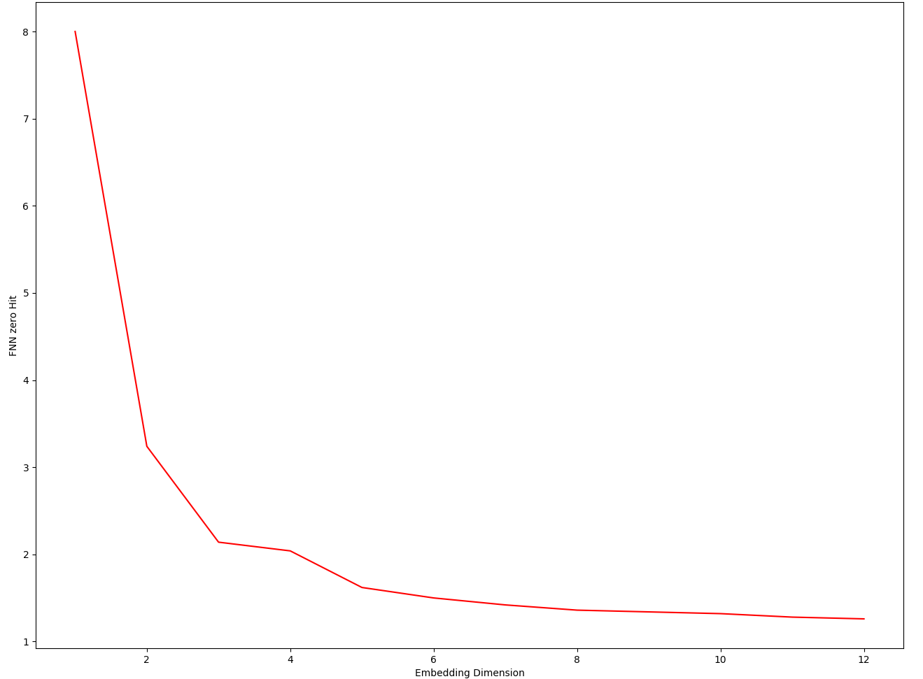
Here, we can see that, after a point, the curve shallows down, that is we can assume that the attractor had fairly unfolded. For getting this value of \(m\), we need to find the knee point of this monotonously decreasing curve. This could be done by choosing a termination criteria like the following:

\[m = \{ \text{max}(m') \mid r_{0}(m'-1) - r_{0}(m') \geq \beta \}\]

Which was implemented using the function findm().

findm()

findm(u, n, d, tau, sd, delta, Rmin, Rmax, rdiv, bound)

Function that finds the value of m whre the r at which FNN ratio hits zero vs m curve flattens(defined by bound value)

Parameters:

• u (ndarray) – double array of shape (n,d). Think of it as n points in a d dimensional space

• n (int) – number of samples or observations in the time series

• d (int) – number of measurements or dimensions of the data

• tau (int) – amount of delay

• m (int) – number of embedding dimensions

• r (double) – ratio parameter

• sig (double) – standard deviation of the data

• delta (double) – the tolerance value(the maximum difference from zero) for a value of FNN ratio to be effectively considered to be zero

• Rmin (double) – minimum value of r from where we would start the parameter search

• Rmax (double) – maximum value of r for defining the upper limit of parameter search

• rdiv (Int) – number of divisions between Rmin and Rmax for parameter search

• bound (double) – bound value for terminating the parameter serch

Returns:

m (double) – value of embedding dimension

References

• Kantz, H., & Schreiber, T. (2004). Nonlinear time series analysis (Vol. 7). Cambridge university press. section 3.3.1

Now we have two important parameters for time delayed embedding, \(tau\) and \(m\).